Hey folks,
Functions in maths is like a machine. A machine that takes an input, does something with that and produces an output.
Let’s take a vending machine as an example. Let’s assume that we don’t need money to buy food from the machine. Just pressing a button will give us the food.
Here the vending machine is the function. It’s output (food) depends on the input (button). If you press a button for soda, you’ll get soda. If you press a button for chips, you’ll get chips.
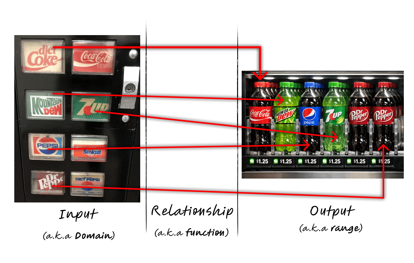
The vending machine maintains a relationship between the input and the output. A function in math is exactly the same.
A mathematical function takes an input (or more than one), performs some operation and produces an output (only one output).
Here, the vending machine has a set of buttons (inputs) that are possible to press. It makes sure that no unexpected input is provided. And it also has a set of food (outputs).
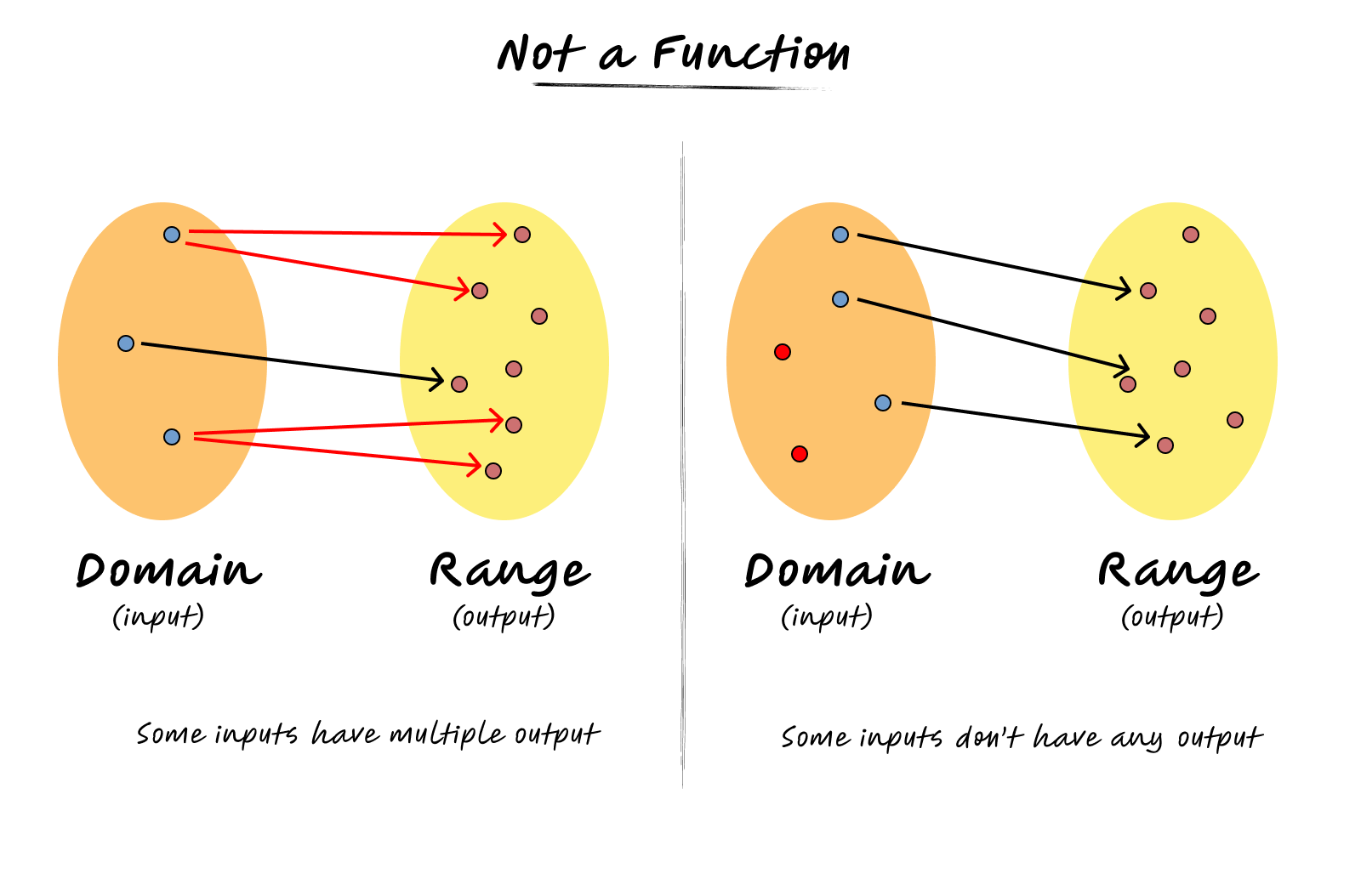
The set of all possible inputs is called the domain, and the set of all possible outputs is called the range. Every input in the domain maps to exactly one output in the range. If one input could produce multiple outputs, it wouldn’t be a function anymore.

It actually resembles functions in programming language. In programming, a function takes one or more inputs and produces only one output. You might argue that we can return an array of values from a function. But still, that array is a single unit that compresses more than one value.
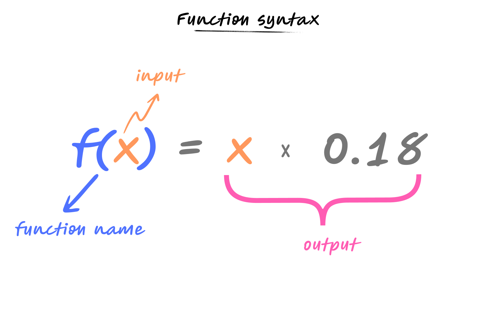
In maths, we write functions as $f(x)$, where $f$ is the name of the function and $x$ is the input. The rule that defines what the function does is written after an equals sign.
The name of a function can be anything, it’s just a label. While $f$ is commonly used, you could use $g(x)$, $h(x)$, or even more descriptive names like $\text{calculate}(x)$ or $\text{tax}(\text{price})$. The choice of name doesn’t change what the function does; it’s just a way to identify and refer to it.
Functions in programming work the same way. They take inputs, perform operations, and return outputs. The mathematical concept directly translates to code.
Let’s create our first function
Let’s say you’re building a checkout system for an online store. When a customer makes a purchase, you need to calculate the tax on their order.
The tax rate is 18%. So if someone buys something for $100, the tax would be $18. If they buy something for $50, the tax would be $9.
How do you express this relationship mathematically?
You could write it out like “tax equals 18% of the price”.
In mathematical terms, 18% means 18 divided by 100, which is 0.18. So tax equals price times 0.18.
We can write this as a function: $$\text{tax}(\text{price}) = \text{price} \times 0.18$$
Or using the standard function notation: $$f(x) = x \times 0.18$$
Where $x$ is the price. This equation tells us the rule “multiply the input by 0.18”.
Now, how do we use this function? When we want to calculate the tax for a specific price, we substitute that value wherever $x$ appears in the function.
Let’s calculate the tax for a price of 10. We write $f(10)$, which means we’re calling the function with the input value 10.
To evaluate this, we take our function $f(x) = x \times 0.18$ and replace every $x$ with 10:
$$f(10) = 10 \times 0.18$$
Now we calculate: $$f(10) = 1.8$$
So the tax for a price of 10 is 1.8.
Let’s try more values:
- $f(50)$: Replace $x$ with 50 → $f(50) = 50 \times 0.18 = 9$
- $f(100)$: Replace $x$ with 100 → $f(100) = 100 \times 0.18 = 18$
- $f(200)$: Replace $x$ with 200 → $f(200) = 200 \times 0.18 = 36$
This is how functions work. You substitute the input value wherever the variable appears, then perform the calculation.
But what if you want to see how the tax changes as the price increases? You’d have to calculate each value individually.
There’s a better way. We can visualize a function.
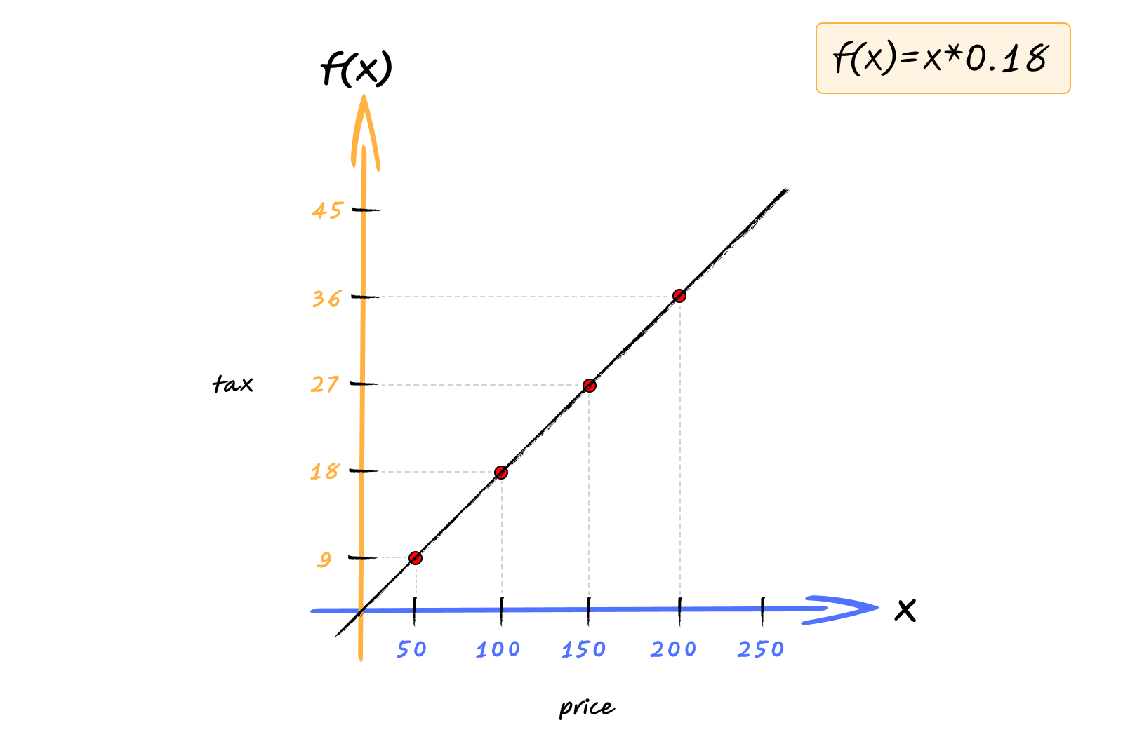
When you visualize a function, you plot it on a graph. The horizontal axis (x-axis) represents the input values (price). The vertical axis (y-axis) represents the output values (tax). For each input, you mark a point where the output would be.
For $f(x) = 0.18x$, you’d plot points like:
- When $x = 0$, $f(0) = 0$, so you mark a point at (0, 0)
- When $x = 50$, $f(50) = 9$, so you mark a point at (50, 9)
- When $x = 100$, $f(100) = 18$, so you mark a point at (100, 18)
- When $x = 200$, $f(200) = 36$, so you mark a point at (200, 36)
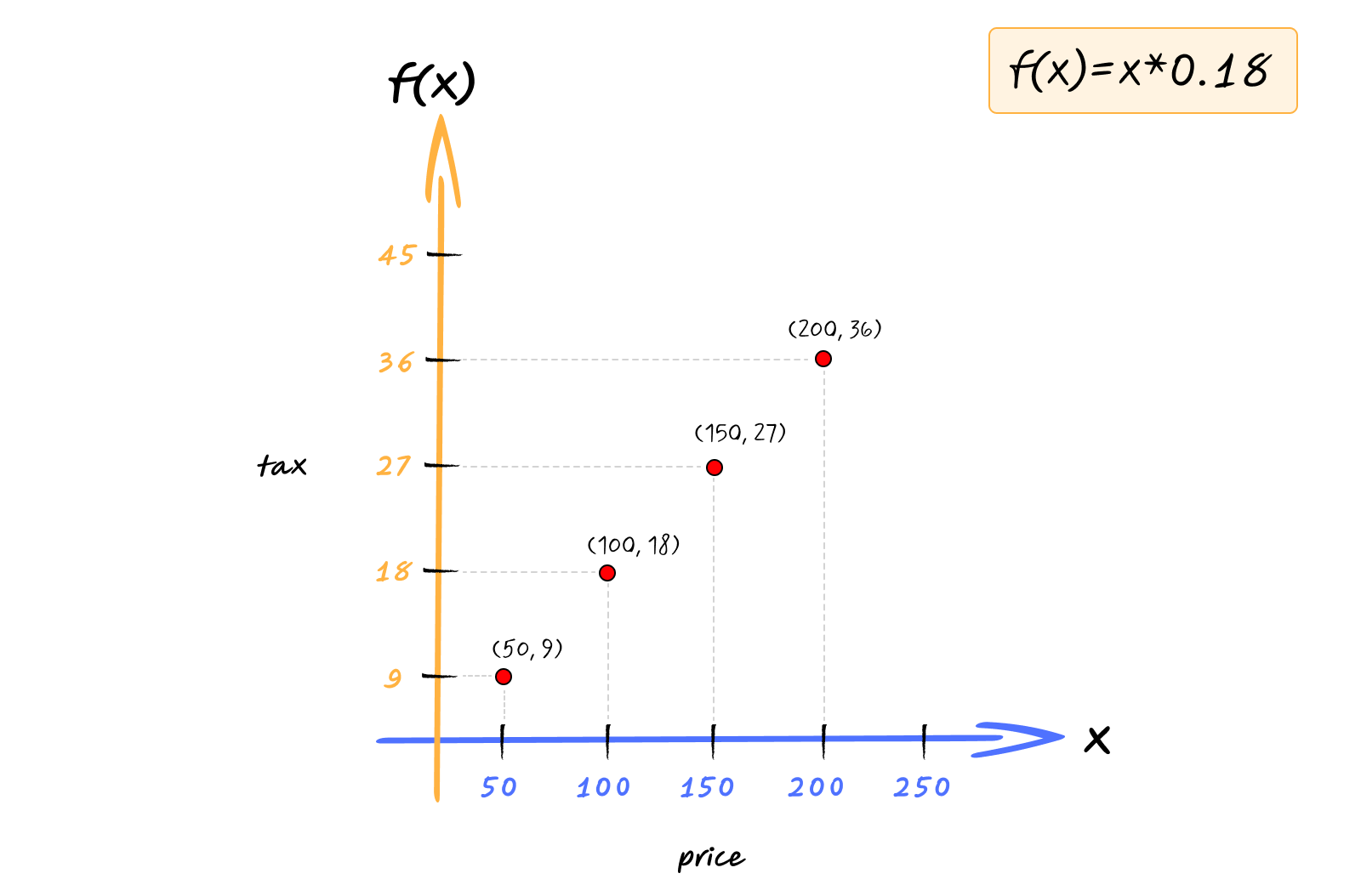
When you connect all these points, you get a straight line that starts at the origin and goes up and to the right.
You can play with this graph here - https://www.desmos.com/calculator/gw82ybjbid
The graph tells you everything at once. You can see that as the price increases, the tax increases proportionally. You can see the line passes through the origin (when price is 0, tax is 0). You can see how steep the line is, the higher the tax rate.
This visual representation makes the function’s behavior concrete. Instead of calculating individual values, you can see the entire relationship at a glance. Different functions create different shapes on graphs, and these shapes help us understand how the function behaves.
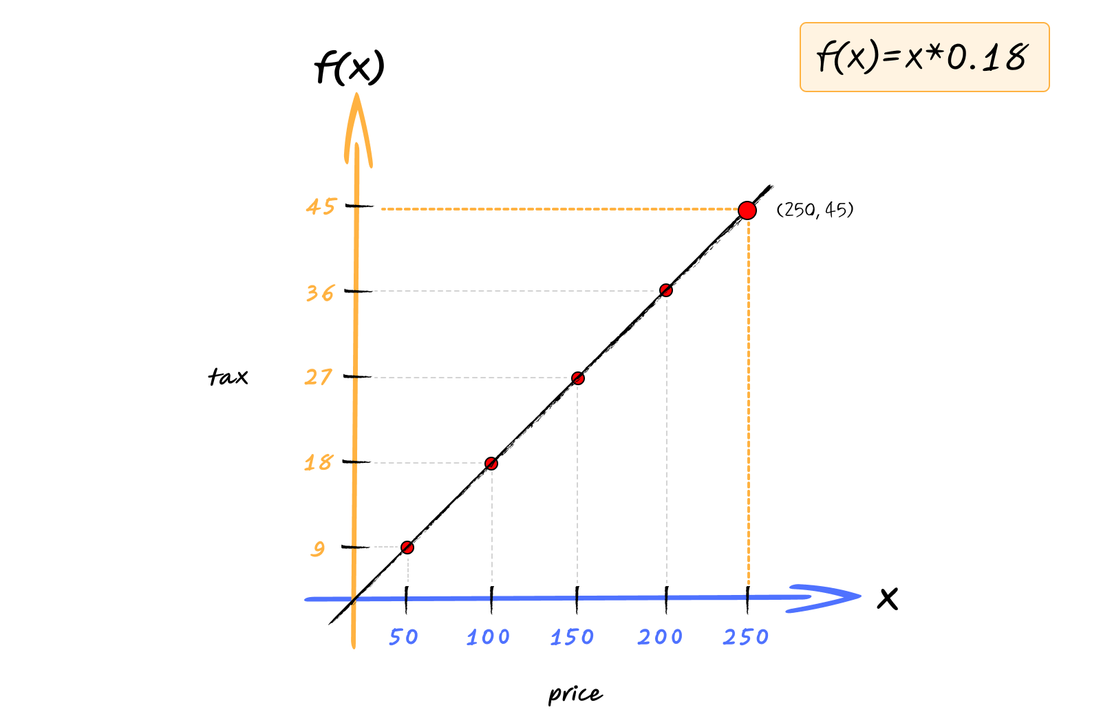
Say if we want to find the tax when price is 250, we can just draw vertical line (dotted orange line) from 250, and an horizontal line (dotted orange line) where the vertical intersects the slanting line (black line).
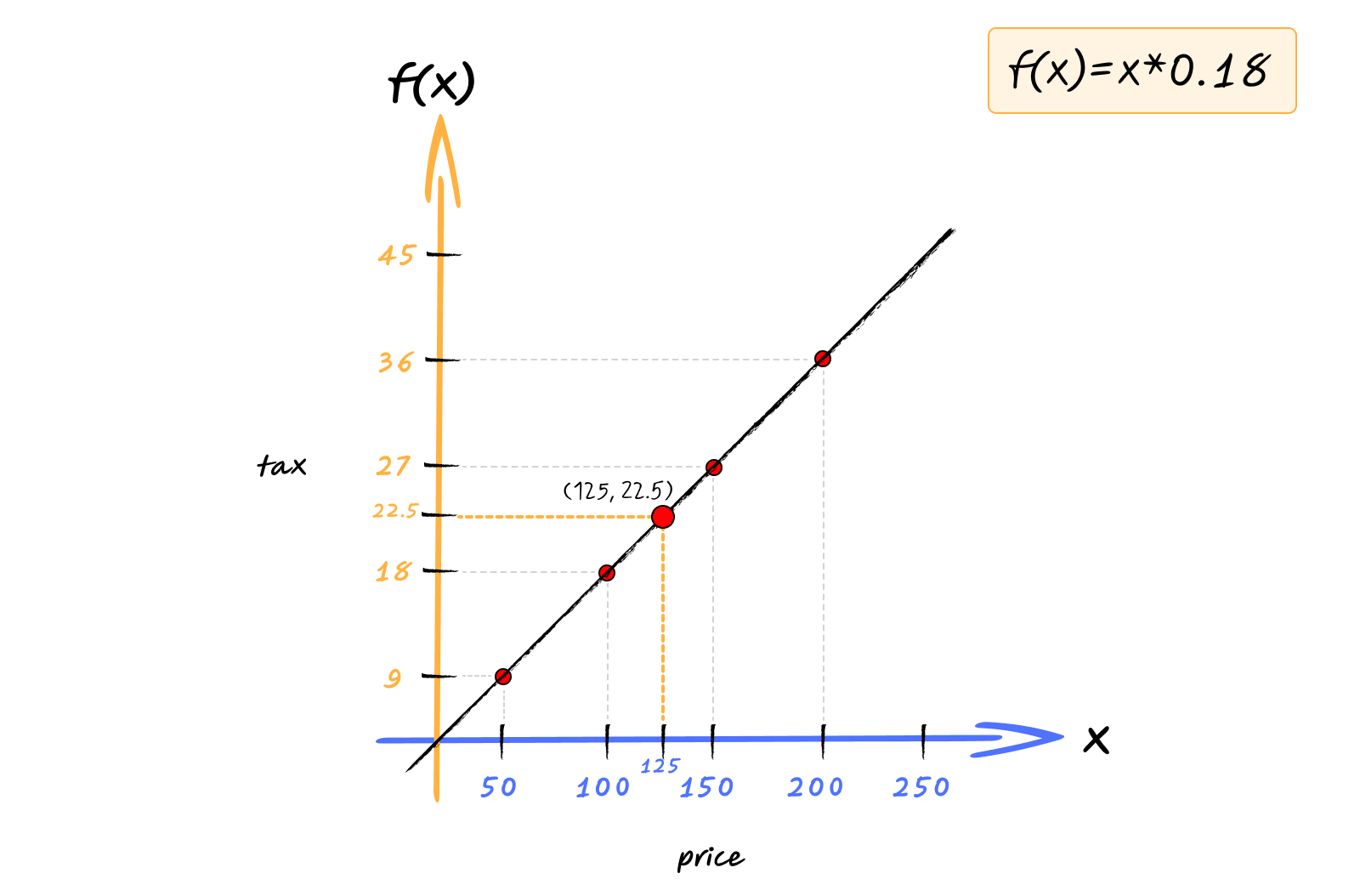
Similarly, if we want to find value for 125,
Now, let’s see how different types of functions solve different kinds of problems.
Linear Functions
Let’s say you want to build a shipping calculator for your e-commerce site.
You’ve analyzed your costs and found a pattern: for every kilogram, you charge $2, plus a fixed base fee of $3 for handling.
How do you model this mathematically?
You could try writing it out case by case. But that’s tedious and doesn’t scale. What you need is a way to express the relationship, “cost equals two times the weight, plus three”.
We can write this as: $$shippingCharge(weight) = (2 \times weight) + 3$$
or simply,
$$f(x) = 2x + 3$$
Where
- $x$ is the weight in kilograms
- 3 is the fixed base fee
Let’s see what this gives us:
- $f(1) = 2(1) + 3 = 5$
- $f(2) = 2(2) + 3 = 7$
- $f(3) = 2(3) + 3 = 9$
- $f(1.5) = 2(1.5) + 3 = 6$
- $f(10) = 2(10) + 3 = 23$

You can play with this graph here - https://www.desmos.com/calculator/czmjkd7bd1
It works for any weight. No need for infinite if-else statements.
Notice something interesting. Every time the weight increases by 1 kilogram, the cost increases by 2 dollars. That’s because we’re multiplying by 2. And no matter what, we always add 3 dollars as the base fee.
What if your costs were different? What if you charge $5 per kilogram with a $10 base fee? Then the function would be:
$$f(x) = 5x + 10$$
Or what if you charge $1.50 per kilogram with no base fee? Then:
$$f(x) = 1.5x + 0$$
Or simply: $$f(x) = 1.5x$$
All of these follow the same pattern, “multiply the input by some number, then add another number (which could be zero)”.
This pattern is so common that mathematicians gave it a name and a general form. We call it a linear function, and we write it as:
$$f(x) = mx + b$$
Here,
- $m$ is the number we multiply by (called the slope)
- $b$ is the number we add (called the y-intercept or base value).
In our shipping example, $m = 2$ and $b = 3$. The slope tells you how much the output changes when the input changes by one unit. The y-intercept tells you the base value when the input is zero.
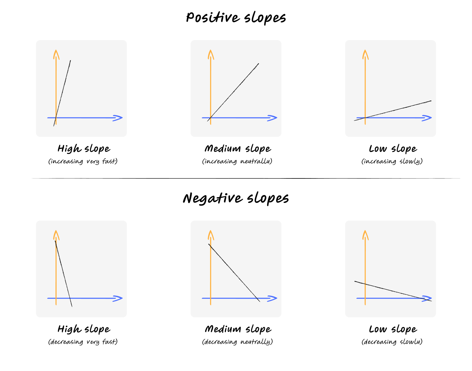
When you graph a linear function, you get a straight line. That’s why it’s called linear. The slope determines how steep the line is, and the y-intercept tells you where it crosses the vertical axis.
Linear functions model relationships where things scale proportionally. Shipping costs, hourly wages, simple interest calculations - all of these follow linear patterns.
Quadratic Functions
Now consider a different problem. You’re building a graphics application, and you need to calculate the area of squares. Given the side length, how do you find the area?
You know the formula - area equals side length times side length.
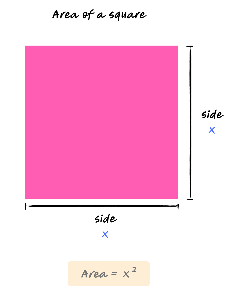
But how do you express this as a function?
You might think, “I’ll just multiply by the side length twice.” That works, but there’s a more elegant way to express repeated multiplication. That is ‘exponents’.
When you multiply a number by itself, you’re raising it to the power of 2.
So instead of writing $x \times x$, you write $x^2$.
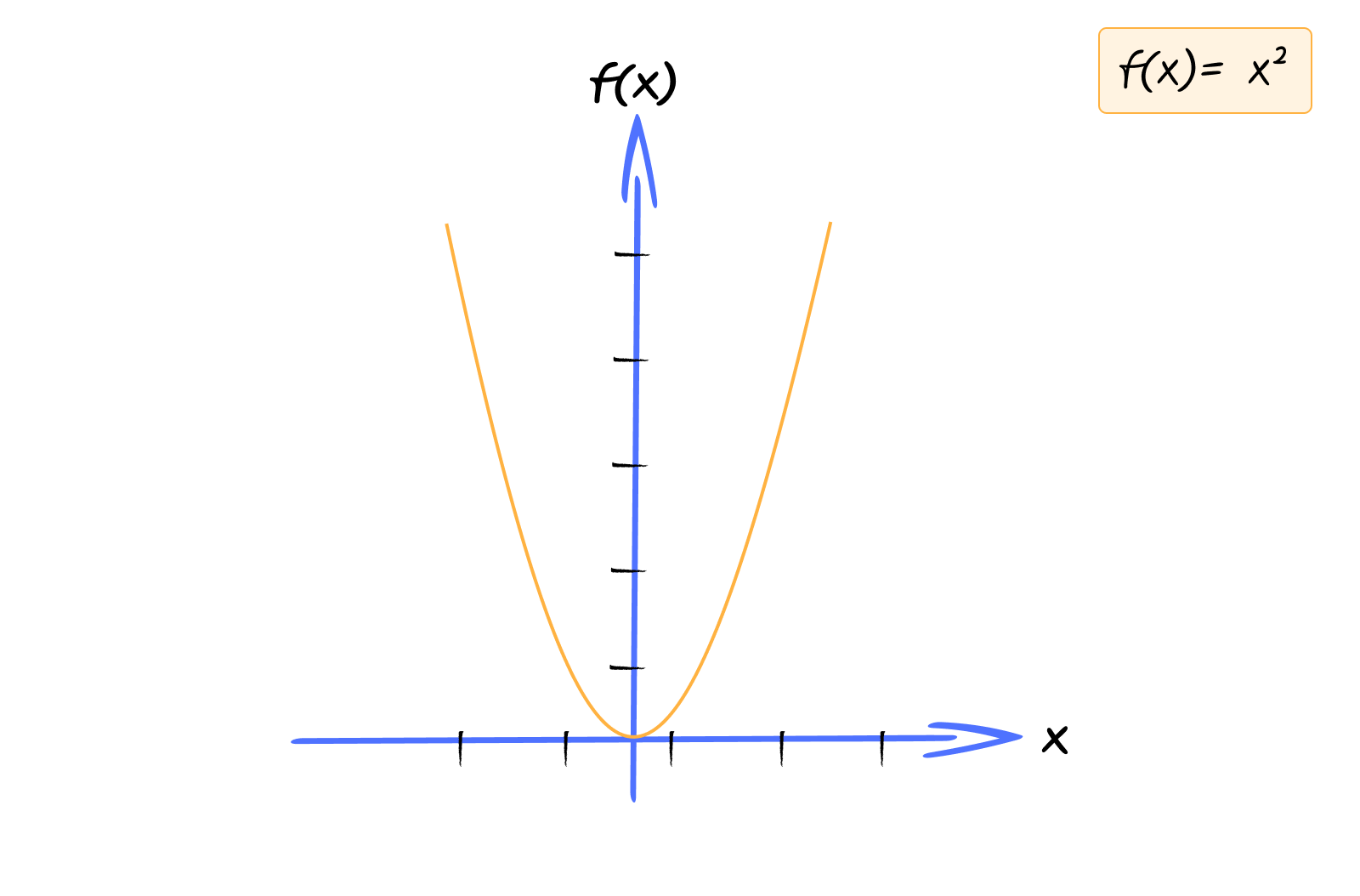
This gives us: $$f(x) = x^2$$
Where $x$ is the side length. Let’s check:
- $f(1) = 1^2 = 1$
- $f(2) = 2^2 = 4$
- $f(3) = 3^2 = 9$
- $f(4) = 4^2 = 16$
- $f(5) = 5^2 = 25$
But here’s something interesting. What happens with negative inputs?
- $f(-2) = (-2)^2 = 4$
- $f(-3) = (-3)^2 = 9$
You can play with this graph here - https://www.desmos.com/calculator/b1hb2plhlf
Negative inputs give the same output as their positive counterparts. That’s because squaring always produces a positive result (or zero).
What if we need something more complex? What if the area calculation involves other terms? For instance, what if we have: $$f(x) = 3x^2 + 2x + 1$$
Let’s see what this gives:
- $f(0) = 3(0)^2 + 2(0) + 1 = 1$
- $f(1) = 3(1)^2 + 2(1) + 1 = 6$
- $f(2) = 3(2)^2 + 2(2) + 1 = 17$
This still involves squaring the input, but now we have additional terms. The highest power is 2 (the squared term), and we can have other terms with lower powers or constants.
All functions that involve squaring the input (and possibly other terms) follow a pattern. We call them quadratic functions, and the general form is:
$$f(x) = ax^2 + bx + c$$
Where $a$, $b$, and $c$ are constants, and $a$ cannot be zero (otherwise the highest power wouldn’t be 2, and it wouldn’t be quadratic).
In our area example, $a = 1$, $b = 0$, and $c = 0$, so we have the simplest quadratic: $f(x) = x^2$.
When you graph a quadratic function, you get a curve called a parabola. It’s U-shaped, opening upward if $a$ is positive, downward if $a$ is negative.
Quadratic functions model relationships where things don’t scale linearly. Area calculations, projectile motion, optimization problems - all of these involve quadratic relationships.
Exponential Functions
Here’s a scenario you might recognize. You’re analyzing user growth for your app.
On day one, you have 1 user. On day two, you have 2 users. On day three, you have 4 users. On day four, you have 8 users.
The number of users doubles every day. How do you model this?
You could write it out: day 1 = 1, day 2 = 2, day 3 = 4, day 4 = 8. But what about day 10? Or day 100? You’d need to double the previous value each time, which gets tedious.
Notice the pattern: day 1 = $2^0 = 1$, day 2 = $2^1 = 2$, day 3 = $2^2 = 4$, day 4 = $2^3 = 8$.
The exponent is always one less than the day number. So for day $x$, you have $2^{x-1}$ users.
But let’s simplify. If we start counting from day 0, then day 0 = $2^0 = 1$, day 1 = $2^1 = 2$, day 2 = $2^2 = 4$. Now the pattern is cleaner: day $x$ has $2^x$ users.
We can write this as: $$f(x) = 2^x$$
Let’s verify:
- $f(0) = 2^0 = 1$
- $f(1) = 2^1 = 2$
- $f(2) = 2^2 = 4$
- $f(3) = 2^3 = 8$
- $f(4) = 2^4 = 16$
- $f(5) = 2^5 = 32$
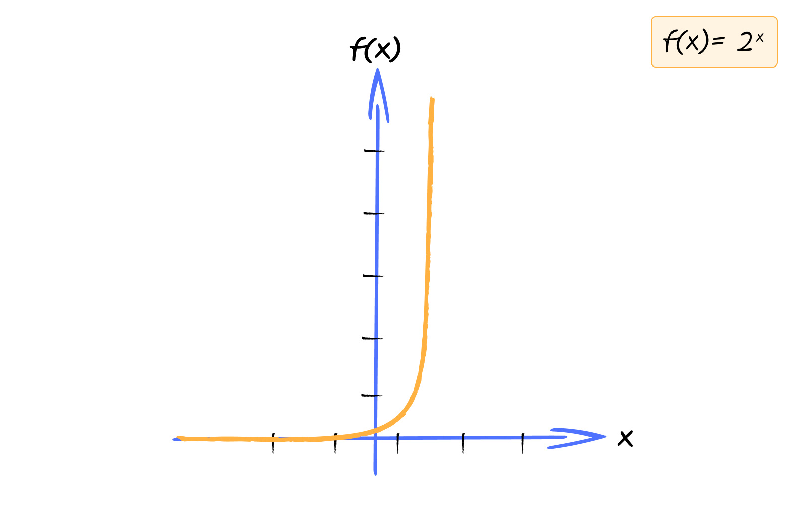
You can play with this graph here - https://www.desmos.com/calculator/c2tanodsry
See how it doubles each time? That’s exponential growth. It starts slow but quickly becomes enormous. By day 10, you’d have $2^{10} = 1024$ users. By day 20, you’d have over a million.
What if the growth rate was different? What if it tripled every day instead of doubling? Then we’d have: $$f(x) = 3^x$$
Or what if it grew by 50% each day? Then we’d use: $$f(x) = 1.5^x$$
All of these follow the same pattern, we raise a constant base to the power of the input variable.
This pattern is called an exponential function, and the general form is:
$$f(x) = a^x$$
Where $a$ is a constant base. The base determines how fast the function grows. With $a = 2$, it doubles each step. With $a = 3$, it triples. With $a = 1.5$, it grows by 50% each step.
Exponential functions model rapid growth or decay. Population growth, compound interest, certain algorithm time complexities, radioactive decay - all of these follow exponential patterns.
In computing, exponential functions show up everywhere. Database growth, network effects, and certain machine learning activation functions all rely on exponential relationships.
Logarithmic Functions
Now consider the opposite question. You have 1024 users, and you know the user base doubles every day. How many days ago did you have just 1 user?
You could work backwards: 1024 → 512 → 256 → 128 → 64 → 32 → 16 → 8 → 4 → 2 → 1. That’s 10 steps, so 10 days ago.
But there’s a more direct way. You’re asking, “what power do I raise 2 to, to get 1024?”.
In other words, $2^? = 1024$.
The answer is 10, because $2^{10} = 1024$.
This is what a logarithm does. It answers the question, “What exponent do I need?”
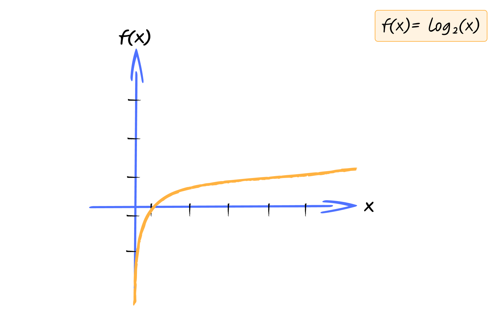
We write this as: $$f(x) = \log_2(x)$$
The subscript 2 is called the base. It tells us we’re asking about powers of 2.
Let’s see what this gives us:
- $f(1) = \log_2(1) = 0$ (because $2^0 = 1$)
- $f(2) = \log_2(2) = 1$ (because $2^1 = 2$)
- $f(4) = \log_2(4) = 2$ (because $2^2 = 4$)
- $f(8) = \log_2(8) = 3$ (because $2^3 = 8$)
- $f(16) = \log_2(16) = 4$ (because $2^4 = 16$)
- $f(1024) = \log_2(1024) = 10$ (because $2^{10} = 1024$)
You can play with this graph here - https://www.desmos.com/calculator/2ccpwyqder
What if we were working with a different base? What if we were asking about powers of 10? Then we’d use: $$f(x) = \log_{10}(x)$$
Or powers of 3: $$f(x) = \log_3(x)$$
All of these follow the same pattern, “we’re asking what exponent we need to raise a base to, to get the input value?”.
This pattern is called a logarithmic function, and the general form is:
$$f(x) = \log_a(x)$$
Where $a$ is the base of the logarithm.
Logarithmic functions grow very slowly. To go from 1 to 2, you need to increase the input by 1. To go from 2 to 4, you need to increase by 2. To go from 4 to 8, you need to increase by 4. The amount you need to increase keeps getting larger, which means the function itself grows slower and slower.
Logarithmic functions are the inverse of exponential functions. If exponential functions model rapid growth, logarithmic functions model slow growth. They answer the question, “How many times do I need to multiply the base to get this number?”
In programming, you’ve probably seen logarithmic time complexity, written as $O(\log n)$. Binary search is a classic example. Each step eliminates half the remaining possibilities. To search through 1024 items, you only need 10 steps. That’s the power of logarithmic scaling.
Polynomial Functions
Sometimes, relationships aren’t simple. They involve multiple terms, different powers, and various constants.
Imagine you’re modeling the trajectory of a ball thrown into the air. The height depends on time, but it’s not just a simple multiplication. Gravity pulls it down, initial velocity pushes it up, and there’s an initial height.
You need a function that combines multiple terms: $$f(t) = -5t^2 + 20t + 10$$
Here, $t$ is time in seconds. The $-5t^2$ term represents the effect of gravity (pulling down). The $20t$ term represents the initial upward velocity. The $10$ is the initial height.
Let’s see what this gives us:
- $f(0) = -5(0)^2 + 20(0) + 10 = 10$
- $f(1) = -5(1)^2 + 20(1) + 10 = 25$
- $f(2) = -5(2)^2 + 20(2) + 10 = 30$
- $f(3) = -5(3)^2 + 20(3) + 10 = 25$
- $f(4) = -5(4)^2 + 20(4) + 10 = 10$
Notice how the height increases, reaches a peak, then decreases. That’s because gravity eventually overcomes the initial upward velocity.
What if we had a simpler polynomial? What about: $$f(x) = x^3 + 2x^2 - x + 1$$
Let’s calculate some values:
- $f(0) = 0^3 + 2(0)^2 - 0 + 1 = 1$
- $f(1) = 1^3 + 2(1)^2 - 1 + 1 = 3$
- $f(2) = 2^3 + 2(2)^2 - 2 + 1 = 15$
Or even simpler, what we’ve seen before: $$f(x) = 2x + 3$$
This is also a polynomial, just with a single term of power 1.
All of these functions combine multiple powers of the input variable. They’re called polynomial functions, and the general form is:
$$f(x) = a_nx^n + a_{n-1}x^{n-1} + \ldots + a_1x + a_0$$
Where each $a$ is a constant coefficient, and $n$ is a non-negative integer called the degree of the polynomial. The degree is determined by the highest power of $x$ in the function.
In our trajectory example: $$f(t) = -5t^2 + 20t + 10$$
This is a second-degree polynomial (also called a quadratic, which we saw earlier). The highest power is 2.
Polynomials can have any degree. A first-degree polynomial is linear (like $2x + 3$). A third-degree polynomial is cubic (like $x^3 + 2x^2 - x + 1$).
Polynomials are flexible. They can model complex relationships by combining simpler terms. Curve fitting, approximation, and various mathematical models rely on polynomials because they can approximate many different shapes.
Constant Functions
Sometimes, you need a function that always returns the same value, regardless of input.
Imagine you’re building a configuration system. Every user gets the same default theme, no matter who they are. The function always returns “dark”.
Or maybe you’re calculating a fixed processing fee that’s always $3, regardless of the order amount.
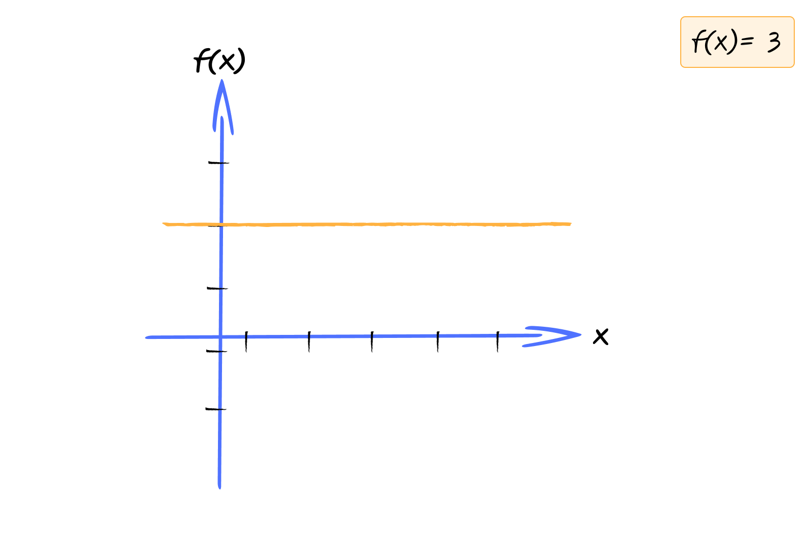
We can write this as: $$f(x) = 3$$
Let’s see what this gives us:
- $f(0) = 3$
- $f(100) = 3$
- $f(-50) = 3$
- $f(1000) = 3$
No matter what $x$ is, $f(x)$ always equals 5. The input doesn’t affect the output at all.
What if the fixed value was different? What if it was always 10? $$f(x) = 10$$
Or always 0? $$f(x) = 0$$
All of these follow the same pattern. The output is always the same constant value, regardless of the input.
This pattern is called a constant function, and the general form is:
$$f(x) = c$$
Where $c$ is a constant value.
When you graph a constant function, you get a horizontal line. It never changes, no matter what the input is.
Constant functions might seem trivial, but they’re useful when you need a fixed value that doesn’t depend on input. Default settings, base configurations, and fixed offsets all use constant functions.
Piece-wise Functions
So far, we’ve seen functions that follow a single rule for all inputs. But what if the rule changes depending on the input value?
Imagine you’re building a pricing system. For orders under $50, you charge a flat $10 shipping fee. For orders between $50 and $100, you charge 5 times the order value. For orders over $100, shipping is free.
In code, you’d write this as:
function calculateShipping(orderValue) {
  if (orderValue < 50) {
    return 10;
  } else if (orderValue >= 50 && orderValue <= 100) {
    return orderValue * 5;
  } else {
    return 0;
  }
}
This is a conditional function. The output depends on which condition the input satisfies.
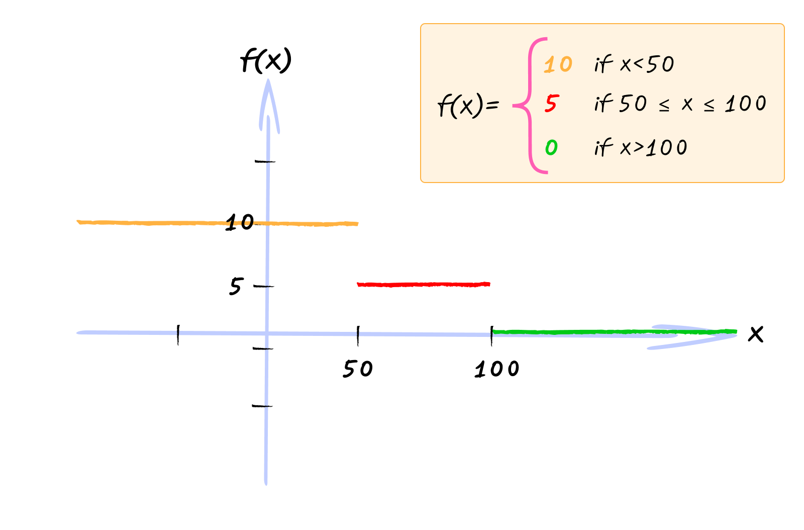
In mathematics, we express this same logic using a piece-wise function. We write different rules for different ranges of input values:
$$ f(x) = \begin{cases} 10 & \text{if } x < 50 \\ 5x & \text{if } 50 \leq x \leq 100 \\ 0 & \text{if } x > 100 \end{cases} $$
The curly brace on the left groups all the pieces together. Each line defines a rule and the condition when it applies.
Let’s verify this works:
- $f(30) = 10$ (because $30 < 50$)
- $f(75) = 5(75) = 375$ (because $75$ is between 50 and 100)
- $f(150) = 0$ (because $150 > 100$)
Each piece of the function applies to a specific range of inputs. When you graph a piece-wise function, you get different shapes in different regions.
You can play with this graph here - https://www.desmos.com/calculator/jifvaus055
Piece-wise functions are useful when relationships change at certain thresholds. Tax brackets, tiered pricing, discount systems, and step functions all use piece-wise logic.
The mathematical notation makes the conditions explicit. You can see exactly which rule applies to which range of values, making the function’s behavior clear and precise.
Multivariable Functions
So far, we’ve only seen functions that take a single input. But what if the output depends on multiple inputs?
Imagine you’re building a shopping cart system. You need to calculate the total cost of an order. The total depends on two things - the price of each item and the quantity purchased.
If someone buys 3 apples at $2 each, the total is $6. If they buy 5 apples at $2 each, the total is $10. But what if the price changes? If they buy 3 apples at $3 each, the total is $9.
The total cost depends on both the price and the quantity. You can’t express this with a single variable.
We need a function that takes two inputs. We write it as: $$f(x, y) = x \times y$$
Where $x$ is the price and $y$ is the quantity. This function multiplies the two inputs together.
Let’s see how we evaluate this. When we call $f(2, 3)$, we’re saying the price is 2 and the quantity is 3. We substitute both values:
- Replace $x$ with 2
- Replace $y$ with 3
So: $$f(2, 3) = 2 \times 3 = 6$$
Let’s try more values:
- $f(2, 5)$: Replace $x$ with 2, $y$ with 5 → $f(2, 5) = 2 \times 5 = 10$
- $f(3, 3)$: Replace $x$ with 3, $y$ with 3 → $f(3, 3) = 3 \times 3 = 9$
- $f(5, 4)$: Replace $x$ with 5, $y$ with 4 → $f(5, 4) = 5 \times 4 = 20$
For two-variable functions, we cannot plot 2D graph like we are doing so far. We can plot a 3D graph to visualize this function better. In 2D graph the value of a function f(x) will be usually placed in y-axis. In 3D graph, the value will be usually placed on z-axis.
You can play with this graph here - https://www.desmos.com/3d/hoduwo9ewj
What if we need even more inputs? Consider calculating the volume of a box. The volume depends on length, width, and height: $$f(l, w, h) = l \times w \times h$$
Where $l$ is length, $w$ is width, and $h$ is height. For a box that’s 5 units long, 3 units wide, and 2 units tall: $$f(5, 3, 2) = 5 \times 3 \times 2 = 30$$
NOTE:
For more than 2 variables, we can’t really plot in 4D or higher. Because, we humans can only perceive maximum of 3-dimensions.
However, we can add more dimensions in different ways like color coding, using different shapes, etc.,
But these are out of topic for this post. If you’re interested in knowing more about plotting higher dimensional functions, search for ‘heatmaps’ and ‘scatterplots’.
Functions that take multiple inputs are called multivariable functions (or functions of several variables). The general form is: $$f(x_1, x_2, x_3, \ldots, x_n)$$
Where $x_1, x_2, x_3, \ldots, x_n$ are the input variables. The function can use any or all of these variables in its calculation.
When you evaluate a multivariable function, you substitute each input value into its corresponding variable, then perform the calculation.
Multivariable functions model relationships where the output depends on several factors. Total cost depends on price and quantity. Volume depends on length, width, and height. Distance depends on speed and time. In programming, you’re already familiar with functions that take multiple parameters are multivariable functions.
The mathematical concept directly translates to code. When you write calculateTotal(price, quantity), you’re using a multivariable function. The syntax is different, but the idea is the same.
One-to-One and Many-to-One
A function can also be called a map. It maps every input to an output. This terminology emphasizes the relationship - each input value is mapped (or connected) to exactly one output value. When we say a function “maps” inputs to outputs, we’re describing how it establishes this connection between the domain and range.
Functions can also be classified by how inputs map to outputs.
Consider the function $f(x) = 2x$. Different inputs always produce different outputs. This is called a one-to-one function (also called injective).
Now consider $f(x) = x^2$. We saw that $f(2) = 4$ and $f(-2) = 4$. Different inputs can produce the same output. This is called a many-to-one function.
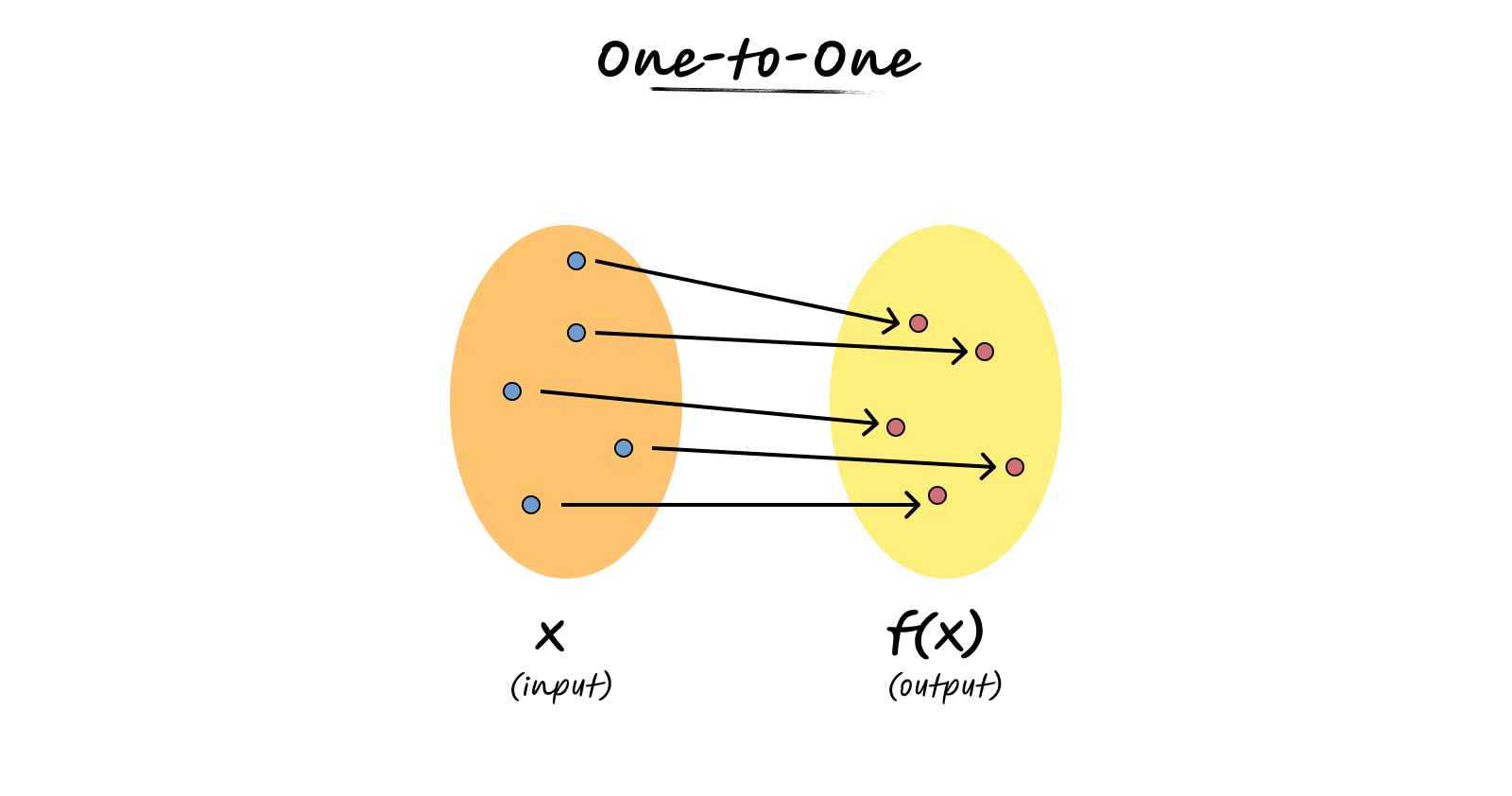
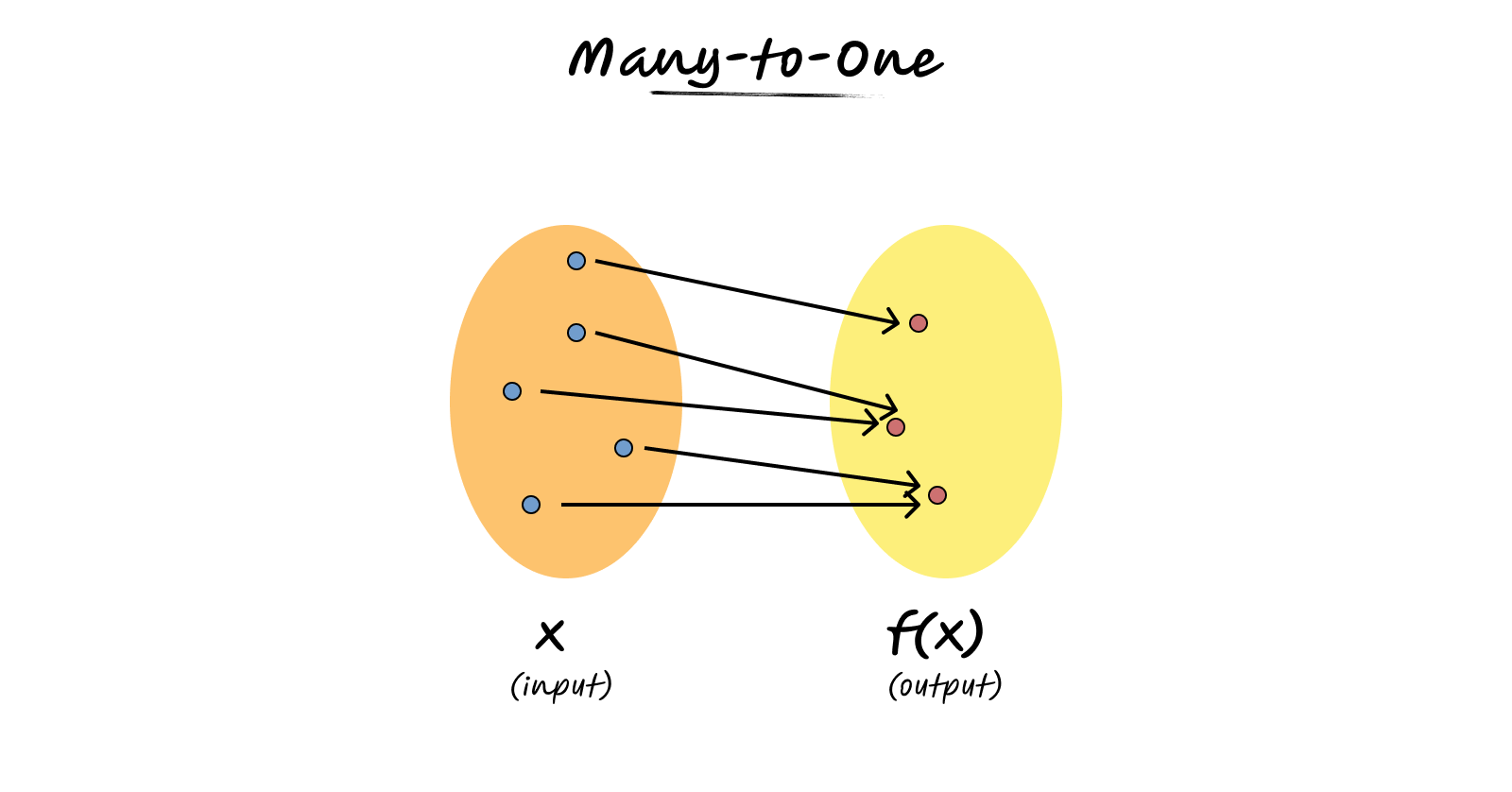
One-to-one functions are useful when you need to reverse the relationship. If each output comes from exactly one input, you can always work backwards to find the original input. Many-to-one functions lose information - you can’t always determine the original input from the output alone.
Why This Matters
Functions aren’t just abstract mathematical concepts. They’re tools for modeling real-world relationships. Every time you write a function in code, you’re using the same mathematical idea.
Understanding different types of functions helps you recognize patterns. When you see a problem that involves proportional scaling, you think linear. When you see area or squared relationships, you think quadratic. When you see rapid growth, you think exponential.
The mathematical foundation helps you choose the right tool for the problem. Instead of writing complex conditional logic, you can express relationships elegantly with functions.
Functions in math are like functions in programming: they take inputs, apply rules, and produce outputs. The syntax might be different, but the core idea is the same.
The next time you encounter a relationship between variables, ask yourself: what function models this? The answer will guide you to a cleaner, more elegant solution.